Plot

1. Methods
2. Colors
3. Line types
4. Legend
5. Layout
6. Axes
7. Grid
8. Endpoint markers (explicit functions only)
9. Implicit functions
10. Custom domains
11. Predefined function types

---

A standard continuous function graph — the smooth curve you’d see in a high-school or calc 1/2 class, as opposed to DiscretePlot’s discrete bars. Plot draws both explicit functions (y = f(x), sampled along x and connected point-to-point) and implicit functions (a relation f(x, y) = 0, traced with Asymptote’s contour module) — mix as many of either kind as you like on one Plot, in the order you add them, by passing the function straight to add(). Colors are assigned automatically once every function is in place: the seven-color rainbow (ROYGBIV) gradient is divided into as many zones as there are functions (explicit and implicit together), and each function takes its zone’s middle color.

Plot is a typedef alias for the underlying ContinuousPlot struct — the two names are fully interchangeable everywhere (variables, parameters, Plot(...)/ContinuousPlot(...) construction). Use whichever reads better; this doc uses Plot.

Define an explicit or implicit function the same way as any other Asymptote function — with the plain real return type, not a real_function_1/implicit_2 alias (those aliases are for parameter and variable types, not for sugar-typing a function definition’s return type):

real cube(real x) { return x*x*x; }                    // explicit — one real input, real_function_1
real circle(real x, real y) { return x*x + y*y - 9; }  // implicit — two real inputs, implicit_2

Plot p = Plot(-4, 4);
p.add(cube);
p.add(circle, color=red, type=DASHED);

Image img = Image();

img.width(10);

img.height(8);
img.padding(0.5);
img.caption_title("Figure 4");
img.caption_text("$x^3$ and $x^2 + y^2 = 9$ on one Plot.");
img.add(p);

add() tells explicit from implicit apart by the function’s own type — cube takes one real, so it’s sampled along x; circle takes two, so its f(x, y) = 0 curve is traced instead. Neither add() call above specifies a domain: by default a function is evaluated (or, for implicit, searched for) across the plot’s own resolved window, since that already defines where you’re looking in the xy-plane — no separate domain bookkeeping needed for the common case. See Custom domains below for the rare case where a function genuinely needs a domain narrower or wider than the window.

Methods

Method	Purpose
Plot(x_min=-5, x_max=5)	Build the plot; also the default window left/right (see below)
add(f, color=AUTO_COLOR, type=SOLID, label="", left_marker=AUTO, right_marker=AUTO, samples=200, x_min, x_max)	Add an explicit function (real_function_1)
add(f, color=AUTO_COLOR, type=SOLID, label="", nx=100, ny=nx, x_min, x_max, y_min, y_max)	Add an implicit function (implicit_2)
legend(height=0)	Build a standalone legend picture (see below)
set_window_left / set_window_right / set_window_bottom / set_window_top(real)	Override one viewport edge
set_window(left, right, bottom, top)	Set all four viewport edges at once
set_grid_delta_x / set_grid_delta_y(real)	Change one grid spacing
set_grid(delta_x=1, delta_y=1)	Set both grid spacings and turn the grid on
set_grid_mode(bool)	Turn the grid on/off without changing its spacing
set_margin_left / set_margin_right / set_margin_top / set_margin_bottom(real)	Override one margin (default 1)
set_margins(real)	Set all four margins to the same value
set_margins(left, right, top, bottom)	Set all four margins independently in one call
set_debug_mode(bool)	Draw bounds

Field applicability of add()’s parameters:

Parameter	Explicit	Implicit	Purpose
color	Yes	Yes	Curve color, or AUTO_COLOR to auto-assign from the rainbow palette
type	Yes	Yes	Line/dash style
left_marker, right_marker	Yes	N/A (not a parameter on the implicit overload)	What to draw at the curve’s true left/right ends
samples	Yes	N/A	Points sampled across the domain — higher is smoother, slower
nx, ny	N/A	Yes	contour()’s search grid resolution — higher resolves thin/complex loops more accurately, slower

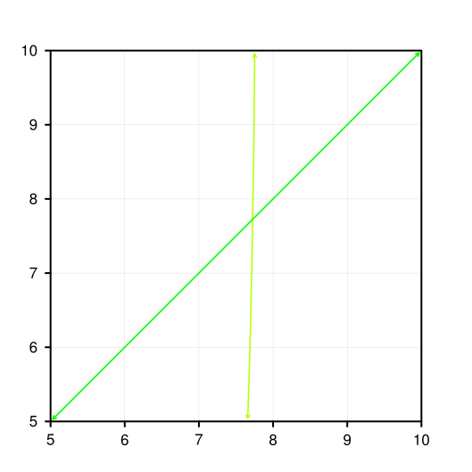
The window (left/right/bottom/top) is the viewport: left/right default to Plot’s own x_min/x_max, and bottom/top are always auto-computed from the sampled y-values of explicit functions only (with padding) unless you override them.

Colors

By default every added function is auto-colored from the rainbow palette (see Styling and typography). Pass any ordinary Asymptote pen — a named color, RGB(...), rgb(...), etc. — as add()’s color argument to color-coordinate a specific function instead:

Plot p = Plot(-3, 3);
p.add(f, color=red);  // f keeps exactly this color
p.add(g);              // g and h are auto-colored, dividing the rainbow between just the two of them
p.add(h);

An explicitly colored function is excluded from the rainbow’s zone count entirely — the remaining auto-colored functions still spread across the full gradient among themselves, rather than losing a slot to a color they don’t use. This applies uniformly to explicit and implicit functions on the same Plot.

Line types

Pass type on add() to set the curve’s dash pattern — one of the constants below, or any other Asymptote linetype pen. type is independent of color, so you can set a line type on an auto-colored function without also having to pin down its color:

Constant	Pattern
SOLID	Solid (default)
DOTTED	Dotted
DASHED	Dashed
LONG_DASHED	Long dashes
DASH_DOTTED	Dash-dot
LONG_DASH_DOTTED	Long dash-dot

p.add(f, type=DASHED);                 // auto color, dashed
p.add(g, color=red, type=DOTTED);      // explicit color and type

Always pass color and type by name (color=..., type=...). They’re both plain pen values in the same add(f, color=AUTO_COLOR, type=SOLID, ...) signature, so Asymptote can only tell them apart by position or by name — color is the first pen slot, so a bare positional pen always fills color, never type. Writing p.add(f, DASHED) intending “set the line type” actually sets color=DASHED, which silently renders as a solid black curve (DASHED carries no color of its own) rather than the dashed line you meant — no compile error, just the wrong picture.

p.add(f, type=DASHED);                  // fine: only type given, named
p.add(f, DASHED);                        // WRONG: silently sets color, not type
p.add(f, type=DASHED, color=red);       // fine: order doesn't matter once named

The line type applies only to the curve itself — an explicit function’s endpoint markers (dots, interval brackets) are always drawn with a solid outline regardless.

Legend

Pass label on add() to name a function; legend(height=0) then builds a standalone legend picture — one row per added function, in add() order, each row a single left-aligned unit: a 2cm line-style sample in that function’s actual color and dash pattern, a small gap, then its label (not two independently aligned columns). A function left unlabeled falls back to "Function N", numbered by its add() order. Colors are resolved the same way render() resolves them (via the same underlying method), so the legend always matches whatever the plot itself actually draws, even for auto-colored functions. Rows are top-aligned: the first added function’s row is topmost, with each subsequent row extending downward.

Plot p = Plot(-10, 10);
p.add(sin, color=blue, label="$\sin(x)$");
p.add(cos, label="$\cos(x)$");   // auto-colored — legend() still shows its resolved color

Image img = Image();

img.width(10);

img.height(10);
img.add(p);

Gallery g = Gallery(1, 2, 10, 10);
g.add(img.pic, 0, 0);
g.add(p.legend(10), 0, 1);       // legend() returns a plain picture, addable like any other

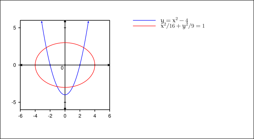
Pass the same height you gave the Gallery/Image to legend(). Gallery.add(picture, ...) always anchors a picture’s bottom-left corner to its cell’s bottom-left corner and expects the picture to fill the whole cell — which a full-size Plot picture does, but a legend, sized only to its own content by default (height=0), doesn’t; left at the default, it ends up hugging the bottom of a much taller cell instead of lining up with the plot. Passing legend()’s height argument to match places the top row at the same margin-inset height the plot’s own square top sits at (height - margin_top), so the two align.

Row spacing, the line sample’s length, and the gap before the label are all theme constants (legend_row_height, legend_line_length, legend_label_gap).

Layout

The actual graph — axes, grid, curves — is drawn inside a square, inset from Plot’s own render area by a margin on each side (set_margin_left/right/top/bottom, or set_margins for all four at once; 1 by default). The square is the largest one that fits after the margins are subtracted, so nothing a Plot draws can ever land outside the area Image gave it — the margins exist specifically to hold tick labels, which always live outside the square, in the margin. Widen a margin if your tick labels are unusually wide and start crowding the edge. The square’s border is drawn last, after every function — so a curve that runs right up to the window’s edge sits underneath the border rather than drawn on top of it.

Axes

Tick marks and their number labels always sit at the square’s own four edges — y-values on the left edge, x-values on the bottom edge, pointing outward into the margin — regardless of where the data axis itself happens to fall. Every tick gets a label, including 0. A data axis line (arrow-tipped) is drawn only when its value actually falls inside the window — an all-positive window like [5, 10] gets no y-axis line at all, just the ordinary edge ticks — and when it is drawn, it also gets small crossing-ticks along it (unlabeled, since the edge already has labels), so it reads the same as a normal graph’s interior axis. When both axes are visible, their true intersection additionally gets a single "0" label of its own, tucked diagonally into whichever quadrant encloses the least area — in addition to, not instead of, the ordinary edge labels.

Grid

Off by default. set_grid(delta_x, delta_y) turns it on and sets the spacing in one call — both default to 1. Grid lines extend across the window, spaced out from 0 (or the window’s edge, if 0 isn’t in view) every delta_x/delta_y; a visible axis’s own position isn’t redrawn as a grid line. Always bounded by the window, so grid lines stay inside the square. Drawn in the theme’s grid_color/grid_thickness, underneath the axes and curves.

Plot p = Plot(-3, 3);
p.add(square);
p.set_grid();              // spacing 1, 1
p.set_grid(0.5, 2);        // override: spacing 0.5 in x, 2 in y
p.set_grid_mode(false);    // turn it back off without losing the spacing

Endpoint markers (explicit functions only)

A function’s true leftmost and rightmost visible points — wherever the curve actually starts and ends, whether that’s the domain edge, a window boundary, or a gap where the function is undefined (e.g. log/sqrt of a negative number) — get a marker, by default (AUTO) an arrowhead. Every other cut in between — an interior window-boundary crossing, or resuming after a gap partway through the domain — always draws with no marker, regardless of left_marker/right_marker; only the two true outermost ends are ever eligible for one. Override left_marker/right_marker on add() when ARROW isn’t right for a specific function — e.g. a closed dot for sqrt(x) at x=0, since it’s actually defined and finite there rather than continuing further:

Constant	Left end	Right end
ARROW (default)	Arrow pointing left	Arrow pointing right
OPEN_DOT	Hollow circle	Hollow circle
CLOSED_DOT	Filled circle	Filled circle
OPEN_INTERVAL	(	)
CLOSED_INTERVAL	[	]
NONE	Nothing	Nothing

Plot p = Plot(-2, 10);
p.add(sqrt, left_marker=CLOSED_DOT);  // sqrt(0)=0 is defined, unlike AUTO's default arrow implies

These only apply to a function’s overall first and last visible point. Any other cut in the middle of the curve — a window-boundary crossing, or resuming after an internal gap — always uses the ordinary AUTO behavior regardless of what you pass here. None of this applies to implicit functions; left_marker/right_marker aren’t even parameters on the implicit add() overload.

An ARROW-marked end has its curve trimmed back by the theme’s plot_arrow_trim (0.1 by default) before drawing, so the arrowhead sits fully inside the window rather than its tip landing exactly on — or poking through — the viewing window’s border. This applies regardless of which edge caused the cut (a window boundary, the domain edge, or a NaN gap); OPEN_DOT/CLOSED_DOT/interval markers are unaffected and stay exactly at the true endpoint.

Implicit functions

An implicit function is a relation f(x, y) = 0 rather than a y = f(x) you can sample along x — a circle (x^2 + y^2 - 9 = 0), for instance, isn’t a function of x at all in the usual sense. Plot traces the curve using Asymptote’s contour module: it searches a box (the window by default) on a grid (nx columns by ny rows) for where f crosses zero, and connects the crossings into one or more paths — which may be closed loops (like a circle), open curves clipped by the box’s edges, or several disconnected pieces, depending on the relation. Because of that, an implicit curve has no equivalent of an explicit function’s “true left/right end,” so it gets no endpoint markers; increase nx/ny (via add()) if a curve’s finer features (thin loops, sharp turns) look faceted at the default resolution.

real circle(real x, real y) { return x*x + y*y - 9; }

Plot p = Plot(-4, 4);
p.set_window(-4, 4, -4, 4);
p.add(circle, color=red, nx=150, ny=150);  // finer grid for a smoother-looking circle

Custom domains

add() always defers to the plot’s own window by default. When a function genuinely needs a domain narrower (or wider) than that — sqrt starting at x = 0 even though the window extends further negative, say — pass x_min/x_max (and, for implicit, y_min/y_max) directly on that add() call:

Plot p = Plot(-2, 10);
p.add(sqrt, x_min=0, x_max=10, left_marker=CLOSED_DOT);   // evaluated over [0, 10], regardless of the window

real circle(real x, real y) { return x*x + y*y - 9; }

Plot p = Plot(-10, 10);
p.add(circle, x_min=-5, x_max=5, y_min=-5, y_max=5);   // searched only in [-5,5]x[-5,5], not the full window

Every bound is independent and optional — set only the ones you need; the rest keep deferring to the window. There’s no separate object to build: the domain lives on the same add() call as everything else, on a per-function basis, independent of the window and independent of every other function on the same Plot.

Don’t confuse this with Plot’s own x_min/x_max (set at construction, via Plot(x_min, x_max)): that’s only the default for the window’s left/right edge when you haven’t called set_window_left/set_window_right — a per-Plot setting, not a per-function one.

Predefined function types

Rather than writing your own implicit relation for common shapes, Utilities/Functions/ provides ready-made ones. Line is the first: a general line in standard form a*x + b*y + c = 0, which — unlike slope-intercept form — represents a vertical line just as naturally as a horizontal or slanted one, since it never divides by anything. as_implicit() exposes it as an implicit_2, which add() accepts directly like any other implicit function:

Line l = vertical_line(5);   // or horizontal_line(y0), line_from_slope_intercept(m, b), line_from_two_points(p1, p2)

Plot p = Plot(-10, 10);
p.add(l.as_implicit(), color=blue);

Constructor	Builds
Line(a, b, c)	The line a*x + b*y + c = 0 directly
vertical_line(x0)	The vertical line x = x0
horizontal_line(y0)	The horizontal line y = y0
line_from_slope_intercept(slope, y_intercept)	y = slope*x + y_intercept (cannot express a vertical line — use vertical_line for that)
line_from_two_points(p1, p2)	The line through two points, vertical or horizontal included

Method	Purpose
evaluate(x, y)	a*x + b*y + c — zero exactly on the line, nonzero (sign indicates which side) elsewhere
as_implicit()	This line as an implicit_2 closure, addable to Plot directly

Conic is the second: a general conic section in standard form A*x^2 + B*y^2 + C*x*y + D*x + E*y + F = 0 — one form covering circles, ellipses, parabolas, and hyperbolas alike, depending on the coefficients:

Conic circle = Conic(1, 1, 0, 0, 0, -9);       // x^2 + y^2 - 9 = 0, a circle of radius 3
Conic hyperbola = Conic(1, -1, 0, 0, 0, -1);   // x^2 - y^2 - 1 = 0

Plot p = Plot(-10, 10);
p.add(circle.as_implicit(), color=blue);

Constructor	Builds
Conic(A, B, C, D, E, F)	The conic A*x^2 + B*y^2 + C*x*y + D*x + E*y + F = 0 directly
conic_circle(center_x, center_y, radius)	A circle
conic_ellipse(center_x, center_y, radius_x, radius_y)	An axis-aligned ellipse
conic_hyperbola(center_x, center_y, radius_x, radius_y, orientation=HORIZONTAL)	An axis-aligned hyperbola
conic_parabola(center_x, center_y, scale, orientation=VERTICAL)	A parabola, from its vertex

These are named with a conic_ prefix rather than plain circle/ellipse, since Asymptote’s own plain library already defines circle(pair, real) and ellipse(pair, real, real) as path constructors — different signatures, but the same bare names would read as if they did the same thing.

orientation (for conic_hyperbola/conic_parabola) is HORIZONTAL or VERTICAL, describing which axis the conic is symmetric about — HORIZONTAL opens left-right, VERTICAL opens up-down (the familiar y = x^2 shape, and conic_parabola’s default).

conic_parabola expresses the parabola in vertex form, with h = center_x, k = center_y, a = scale:

orientation	Equation	Opens
VERTICAL (default)	y = a(x - h)^2 + k	Up if a > 0, down if a < 0
HORIZONTAL	x = a(y - h)^2 + k	Right if a > 0, left if a < 0

(center_x, center_y) is the vertex (h, k); scale (a) is that equation’s leading coefficient — larger magnitude means a narrower parabola.

Conic c = conic_circle(0, 0, 3);                    // x^2 + y^2 = 9
Conic h = conic_hyperbola(0, 0, 2, 3, VERTICAL);    // opens up-down
Conic p = conic_parabola(0, 1, 0.5);                // vertex (0,1), y - 1 = 0.5*x^2, opens upward

Plot plot = Plot(-10, 10);
plot.add(p.as_implicit(), color=blue);

Method	Purpose
evaluate(x, y)	A*x^2 + B*y^2 + C*x*y + D*x + E*y + F — zero exactly on the conic, nonzero elsewhere
as_implicit()	This conic as an implicit_2 closure, addable to Plot directly